Cassie Micucci

Mathematician and Data Scientist

“Data will talk if you’re willing to listen to it.” – Jim Bergeson

Solving problems and analyzing data are my main two things. I am a fifth year graduate student planning to graduate in May 2020 at the University of Tennessee, Knoxville, and I am working on a Ph.D. in Mathematics and an M.S. in Statistics. My advisor is Vasileios Maroulas. My research interests include computational statistics, foundations of data science, data mining, and machine learning. My current research centers on topological data analysis, which combines the mathematical subject of topology with data science and statistics. I have worked on applications in materials science, neuroscience, chemistry, and biochemistry.

Research

My research employs topological data analysis (TDA) for supervised learning tasks on complex data sets and develops statistical and mathematical theory for TDA. TDA uses topology to create powerful tools for the analysis of data by uncovering latent shape present within the data, even despite noise. By condensing a dataset to its most relevant structural qualities, TDA can also reduce data dimension. I have published research that provides applications of TDA in materials science and am preparing papers that leverage TDA to solve problems in chemistry and biochemical engineering. Additionally, using data mining techniques, I have found statistically significant relationships in psychological performance data for the Army Research Laboratory. My research is currently funded by the Army Research Office. Read below to learn more.

What is topological data analysis?

TDA uses topology, specifically homology, to study holes and connected components in data. The clustering of data, along with the empty space (holes, voids) in a dataset provides key information that can help with different data problems.

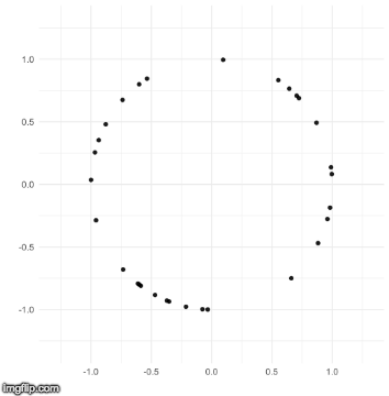
The TDA that I use is called persistent homology. Notice how the black points on the left roughly form a circle. By expanding grey disks centered at each point, eventually the disks connect into an actual circle with a hole in the middle. This moment is called the “birth” of the hole. The hole eventually will disappear when the disks get big enough to fill in the hole – this is called the “death” of the hole.

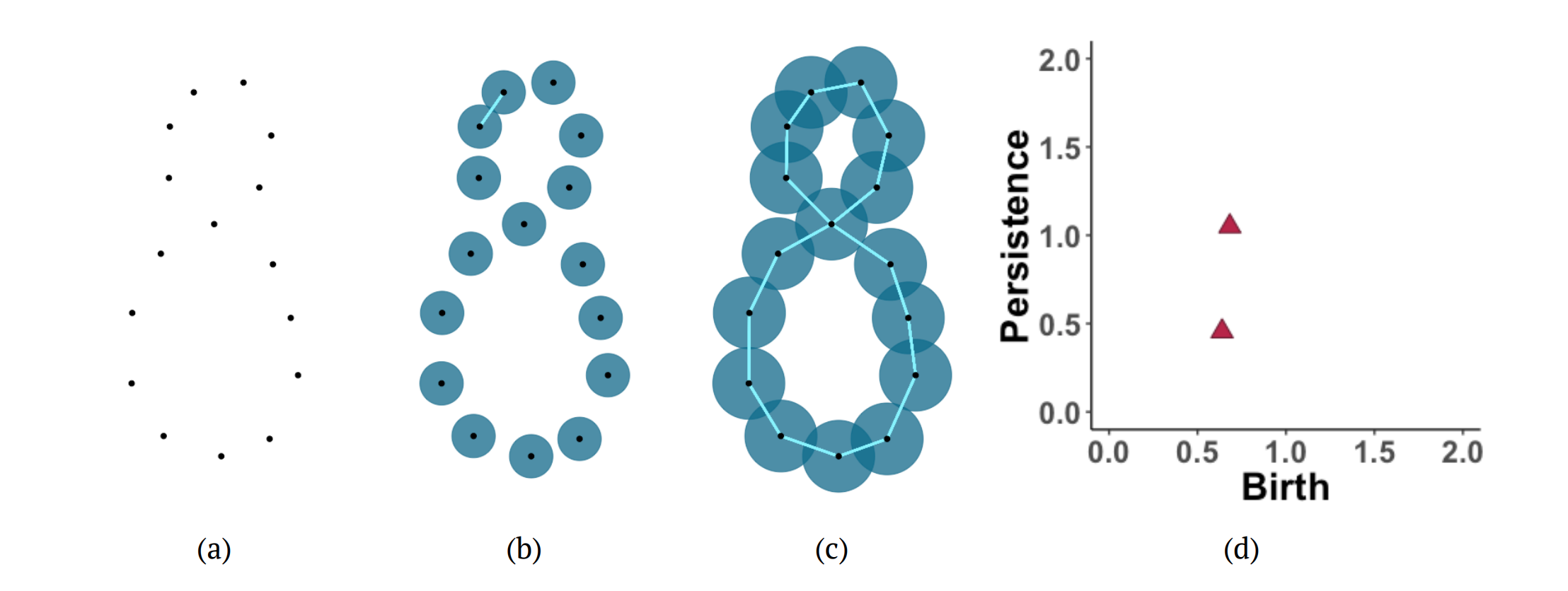
The figure below shows another example of persistent homology. Consider a sample from a figure eight shape (a). After increasing the radius of the balls around the points, a line segment is added in the Vietoris-Rips complex corresponding to the first intersection of balls (b). Eventually, the radius increases so that more line segments are added and two 1-dimensional holes form (c). (d) The persistence diagram provides a visual summary of the evolution of the homology of the data as the radii of the balls increase. The diagram plots when each homological feature appeared (birth) and how long it lasted (persistence).

Distances Between Persistence Diagrams Persistent homology studies holes and connectedness present in data. The clustering patterns of data, along with the empty space (holes, voids) in a dataset, provide key insight into different data problems. Persistent homology provides a process in which a discrete set of points in $\mathbb{R}^n$ can be transformed into a continuous object whose shape can be studied. See the figure above for an example of uncovering 1-dimensional holes (in this example, from the two loops of the figure eight); this procedure can be visualized using balls of increasing radii. The figure shows that TDA can reduce the complexity of a dataset and can expose the most relevant features of the data's shape. Due to this ability, TDA can be utilized in a variety of fields including aviation, physics, neuroscience, astronomy, and genomics. Once computed from data, the persistence diagram can be used as a summary of the data in machine learning tasks, instead of using the original data. For example, a distance on the space of persistence diagrams enables distance-based classification and clustering techniques standard in statistical learning. One aspect of my research focuses on properties and applications of the $d_p^c$ distance for persistence diagrams, first proposed by Maroulas and Marchese as an alternative distance to the traditional Wasserstein distance. The $d_p^c$ distance between diagrams $X = \{ x_1, \ldots, x_n \}$ and $Y = \{ y_1, \ldots ,y_m\}$ is $$ d_p^c(X,Y) = \left( \frac{1}{m} \left( \min_{\pi \in \Pi_m} \sum_{\ell=1}^n \min(c,\|x_{\ell}-y_{\pi (\ell)} \|_{\infty})^p + c^p |m-n| \right) \right)^{\frac{1}{p}},$$ where $\Pi_m$ is the set of permutations of $(1, \dots, m)$. If $m < n$, define $d_p^c (X,Y)$ to be $d_p^c (Y,X)$. This distance measures how well the points in one diagram match the points in the other. It also includes a term which incorporates the difference in the number of points of the two diagrams. The parameter $c$ in the $d_p^c$ distance formula determines how much weight the difference in number of points between the two diagrams is given. For an interactive illustration of this distance and the effect of changing the values of $c$ and $p$, see below.

For more information on this distance for persistence diagrams and an application on time series, see the paper by Marchese and Maroulas. For another application of this distance on materials science data, see this joint work with Spannaus and Maroulas. You can see how this distance works by using the interactive app below.

In a recent work I prove that this distance is stable, a property which ensures that the mapping from a point cloud to the persistence diagram of its Vietoris-Rips complex is continuous under this distance. This continuity is valuable because it guarantees that small perturbations in the underlying points used to create the persistence diagram correspond to small perturbations in this distance between the persistence diagrams. I also derive bounds for the size of the persistence diagrams, both theoretically using graph theory and statistically using a weighted least squares regression. As an application of this distance, we classify the structure of synthetic materials science data as one of two classes, either face-centered cubic or body-centered cubic, with near perfect accuracy. This accuracy is higher than that achieved by using the Wasserstein distance, the standard distance for persistence diagrams. This paper has been submitted to Advances in Data Analysis and Classification, is under review, and is joint work with Professor Vasileios Maroulas and Adam Spannaus.

A future research interest of mine is determining the optimal choice of the constant c in this distance formula given certain properties of the data.
This knowledge will improve classification schemes using this distance by enabling a bypass of brute force searches for the best c over the training set.
Such a result will also reduce the computational burden of the problem and also potentially improve classification results.

Application-Driven Topological Vectorizations

As another approach, one can turn a persistence diagram into a vector and use a standard machine learning method. The persistence image is a well-known method for creating finite dimensional vectors to represent persistence diagrams. Persistence images calculate pixel values of the image through Gaussian distributions centered at points of the persistence diagram; however, it lacks application-specific knowledge in the vectorization. To address this problem, Professor Vasileios Maroulas and I, along with our collaborators in the UTK chemistry department, have developed the application-driven persistence image, which incorporates domain knowledge into the creation of the persistence image.

To apply this method, I developed an algorithm and implemented code in Matlab and R for the prediction of CO₂ and N₂ binding energies for a large dataset of molecules. Accurate prediction of these binding energies aids scientists in the identification of optimal materials for carbon capture technologies. For this application, I use element-specific information to incorporate the identity of the atoms into the Gaussian kernels used to create the image. The images are then used as input to a regression method to predict the binding energy. This method has competitive performance with existing methods on computationally optimized molecules and superior predictions on nonoptimized molecules, offering a way to bypass the computationally intensive optimization step. This research is ongoing.

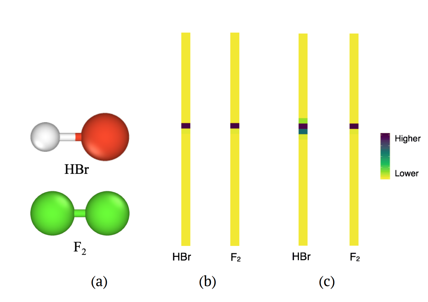
Figure on the right: Molecules HBr and F₂ have the same bond lengths between atoms, resulting in exactly equal features in the persistence diagram. (b) If no chemical information is incorporated, the input vectors from the persistence images are exactly the same. (c) Using our method the input vectors for the molecules in (a) are distinguished by the larger values in several components of the vector for HBr.

Bayesian Inference for Persistent Homology using Cardinality

Persistence diagrams, modeled as point processes, are also amenable to Bayesian inference. By making only very general assumptions about the structure of the underlying point process (i.i.d. clusters), we develop a Bayesian paradigm for persistence diagrams to estimate both the posterior spatial distribution and the posterior distribution of the number of points. This posterior calculation includes terms to account for points that appear or disappear due to noise present in the data. Taking the prior spatial distribution as a Gaussian mixture, we derive the posterior distribution and show that it is a Gaussian mixture as well. We also derive the distribution of the number of points from a binomial prior distribution.

For this Bayesian framework, I have developed a noise distribution that accounts for the specific behavior of noisy points in persistence diagrams.
Also, I have devised a way to adjust the Bayesian calculations for classification applications to account for differences in the number of points between classes.
I have also contributed to the derivation of the posterior equations.

I have written the code in R to apply this Bayesian analysis to the study of filament networks of plant cells. Protein filaments determine the structure, shape, and motion of a cell. Each filament network consists of the locations of actin protein filaments present within the cell. A filament network classification scheme provides researchers with greater insight into the mechanisms which underlie cytoplasmic streaming and intracellular transport. In our Bayesian classification of filament networks, a training set of persistence diagrams generated from each class of filament networks is used to approximate the posterior distribution for each class. The probability that a test persistence diagram belongs to a particular class is then estimated and used to predict the most likely class. This work is ongoing with Professor Vasileios Maroulas, Farzana Nasrin, and collaborators working in biochemical engineering at UTK.

Army Research Lab

As an intern for the summer of 2018, I worked at the Army Research Laboratory (ARL) in Aberdeen, MD through a contract with Thor Industries. There I analyzed data collected from baseball players’ on-field performance and use of a baseball training app. Using machine learning regression techniques, I can predict elements of players’ on-field performance from that within the app. Such predictions of performance aid researchers in developing virtual training for real-life scenarios. I gave an oral presentation as a graduate finalist at the ARL Summer Student Symposium in 2018 based on this research.

Teaching

At the University of Tennessee, Knoxville I was a teaching assistant in a flipped classroom for:

Math 119 (College Algebra)
Math 125 (Basic Calculus)

Also, at UTK I taught and was the instructor of record for:

Math 115 (Statistical Reasoning)